Convexity often arises naturally in many “intuitively” greedy problems. We’ll first give some examples, then go over typical strategies for proving convexity, as well as how to take advantage of it.
Examples
You are given an array of integers. Select distinct indices such that the sum of at those indices is minimized.
It’s not difficult to see that the answer is convex in .
You are given an array of length . If you place exactly tiles of length without overlap, what’s the maximum sum of values that can be covered? (AtCoder)
(note that the first example is just this problem with ) Convexity is a little harder to prove here, but it still makes intuitive sense: with each new tile we add, the total sum gained should be less.
You are given a weighted tree, and some edges are labelled. Find the total weight of an MST that uses exactly edges. (QOJ)
Again, we may suspect that will look something like a parabola, but this will be the hardest proof of the three example listed.
Proof Strategies
Interpolation
The idea of this strategy is to show that if we have solutions of size and with costs and respectively, we can construct a solution of size with cost (or , depending on the problem).
Let’s apply this approach to the second example. First, consider . Let’s draw two valid solutions, one for and one for , as follows:
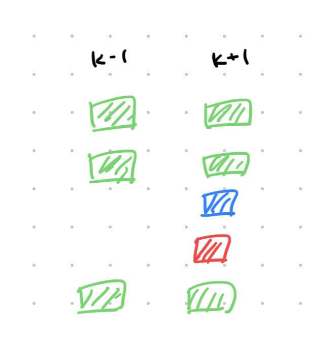 Green tiles are tiles common to both solutions.
Note that if we move the larger of the red and blue tiles over to the solution, the resultant solution will have size and sum .
For , we have to be a bit more clever. Consider the following:
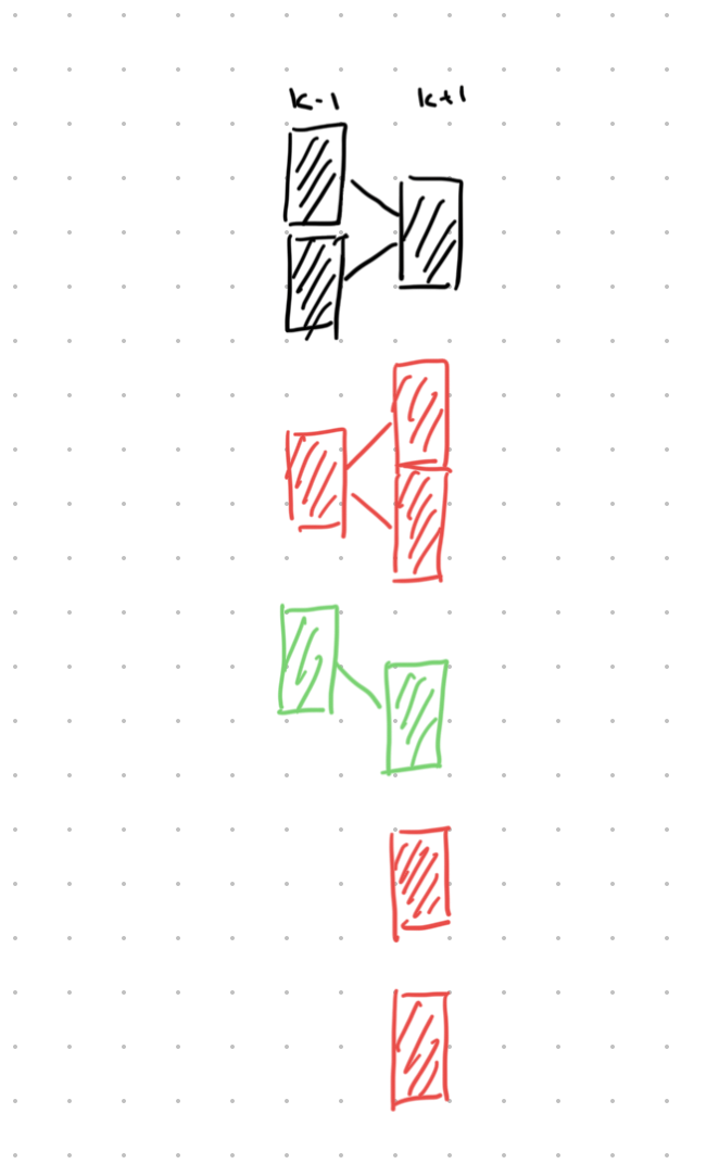 Edges are drawn between overlapping tiles. Note that each component forms a zig-zag pattern.
Our claim is that there exists two optimal solutions for and such that all components are either green (equal # of tiles on left and right) or red (one more tile on right). Assuming this is true, there will be exactly two red components, and we can toggle the one with larger net gain to achieve .
Proof of assumption: If there exists a black component , consider any other red component . Toggle both and in the solution (that is, replace the tiles in the left sides of and with the tiles on the right sides of and ). This cannot change the cost of the solution, otherwise one of the two solutions would not be optimal. Thus and remain the same while one black component is removed; repeat until no black components remaining.