A bit of linear algebra.
An eigenvector of a linear transformation satisfies the relation for some . In other words, only affects the length of its eigenvectors and leaves their direction unchanged.
Note
This idea extends to other linear operators too, not just matrices! For instance, the function is an eigenfunction of the derivative operator .
Matrices
Consider for some matrix . We want to solve the equation . This equation only has non-trivial solutions if , so we just need to solve this for .
2x2 Trick
I’ll give a visual explanation for the neat trick shown here for computing eigenvectors.
First, note that if , the row vectors of must be collinear, like:
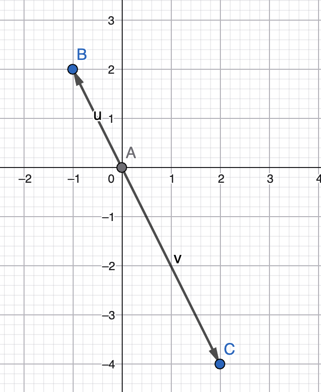 B and C are the row vectors.
Then, note that the set of vectors that are mapped to are precisely the ones perpendicular to both and , i.e. the ones that lie along the blue line:
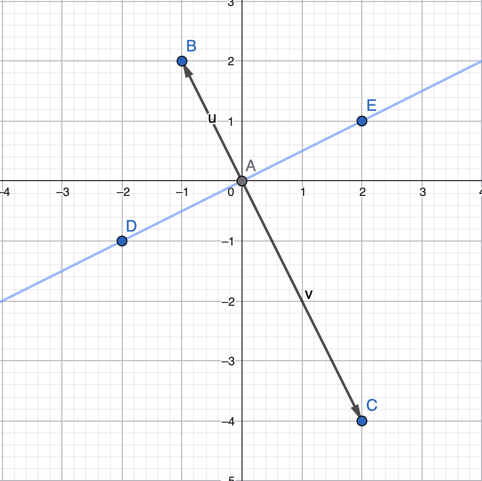
To finish, note that if , then will lie along this blue line. Thus, since , the vector lies along the line. Similarly, also lines on the line. If either of these is not , we’ve found the eigenvector corresponding to .
Imaginary Eigenvalues
Consider the pair , , where are vectors (note that if the matrix itself has only real entries, there must exist a corresponding eigen-pair ).
How can we visualize the trajectory defined by the pair using only the real plane? For instance, when , the corresponding trajectory is just a stretch or shrink along the direction of .
To visualize complex , let’s go into the basis . Note that in this basis, our transformation matrix becomes
This is because we have . Thus,
as desired.
Now, analyzing the polar form of , we see that it satisfies
thus
So, the trajectory that starts at becomes the trajectory